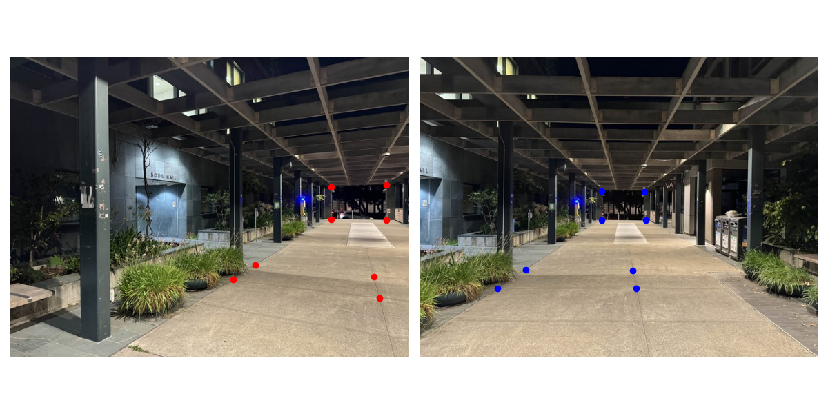
The first part of this project was to shoot pictures. I was kind of lazy about this so I just shot some pictures of my room and of Soda. The most important part about this step is to make sure that when taking the pictures, we should only rotate the camera around its axis, and not do any translations. This is because otherwise it becomes impossible to find a common surface to which we can project the images onto, and there will be no affine transformation. I shot three images for each mosaic, making sure to keep at least 40-70% image overlap for each camera rotation. I then defined correspondences between sequential images using the tool from project 3.

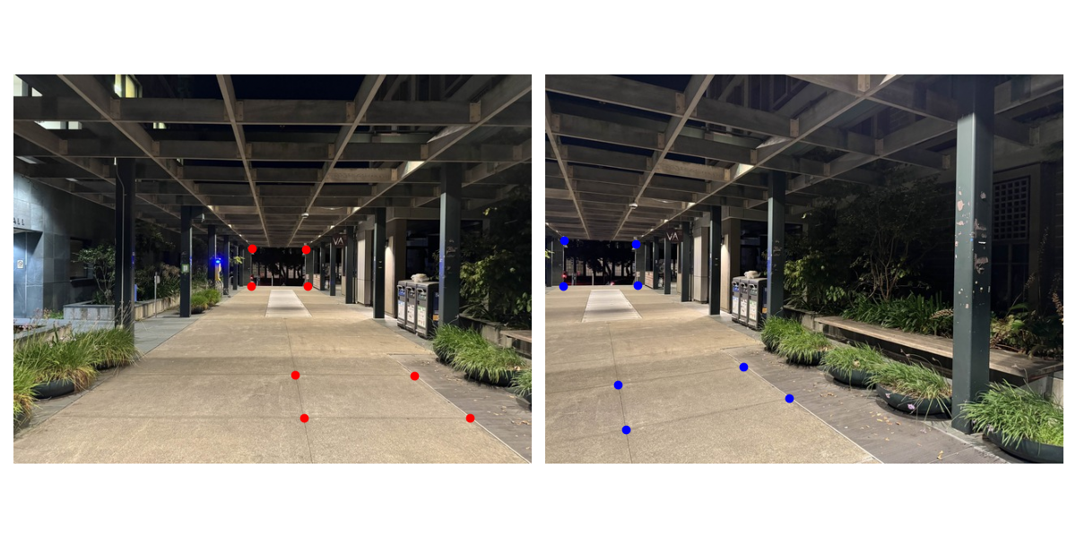
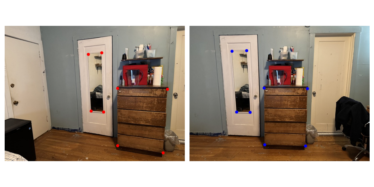
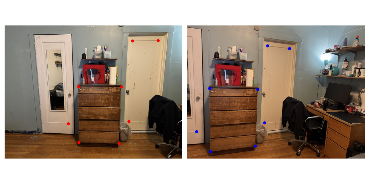
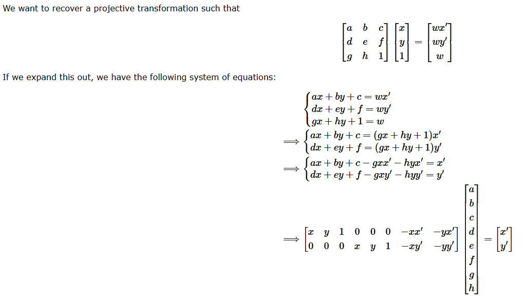
Using the correspondences defined above, we can calculate an affine transformation matrix to go from one image to another. Below is an image explaining how we calculate the transformation matrix given the correspondence points.
The next task is to actually apply the homographies to the relevant images and warp them into the space of the reference image.
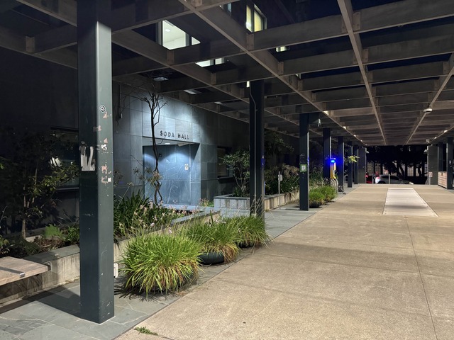
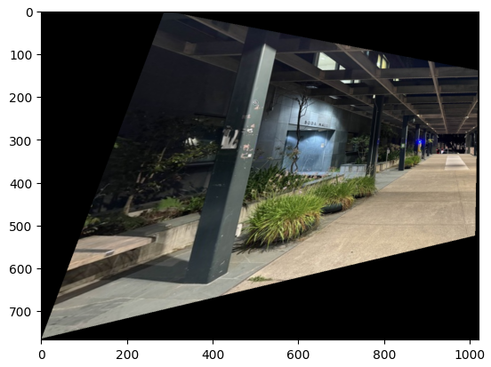
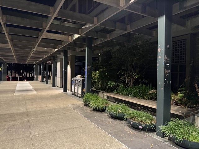
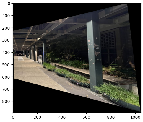
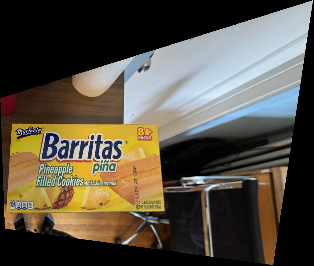
To test out my warp function, I rectified some objects by selecting the corners of the objects and then setting the correspondences to some box like (0,0), (100, 0), (100, 100), (0, 100). From here I calculated the relevant homography for my warp function.
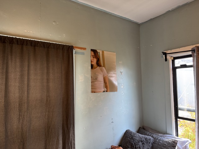
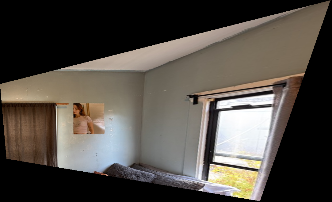
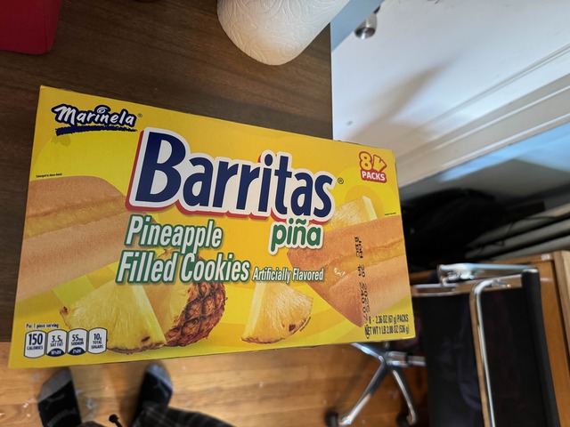
This part required us to align the warped images with the reference image and create a mosaic. My naive approach was just to:
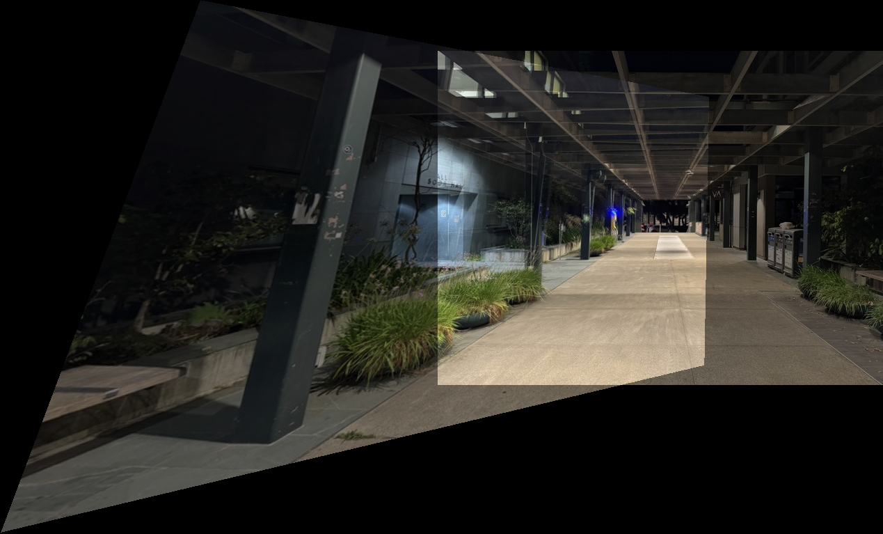
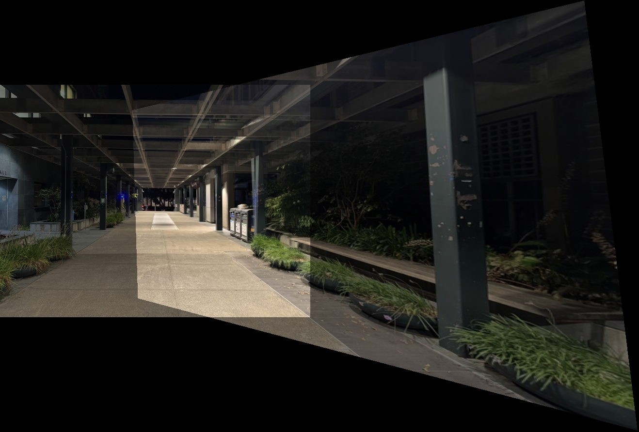
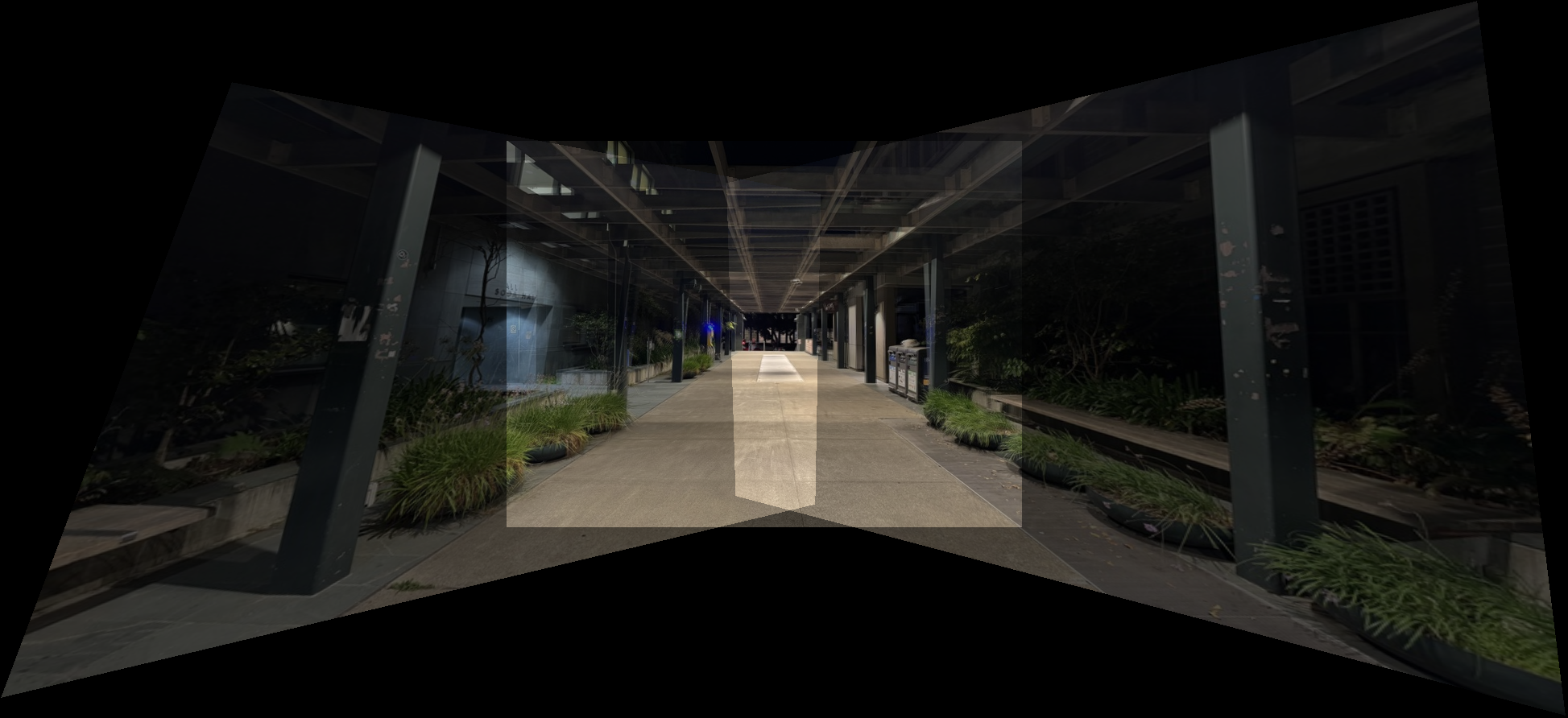
To solve these issues, I used Laplacian blending from project 2 instead of just overlaying the images on top of each other. For the mask, I just had a binary mask where the split point was in the middle of the overlapping region of the images. This greatly improved the quality of the mosaic and removed almost all artifacts. Here are 3 examples below:
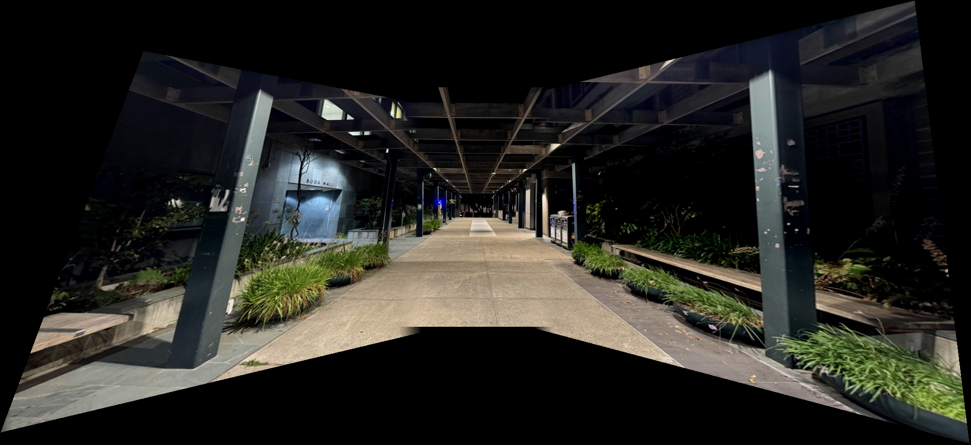
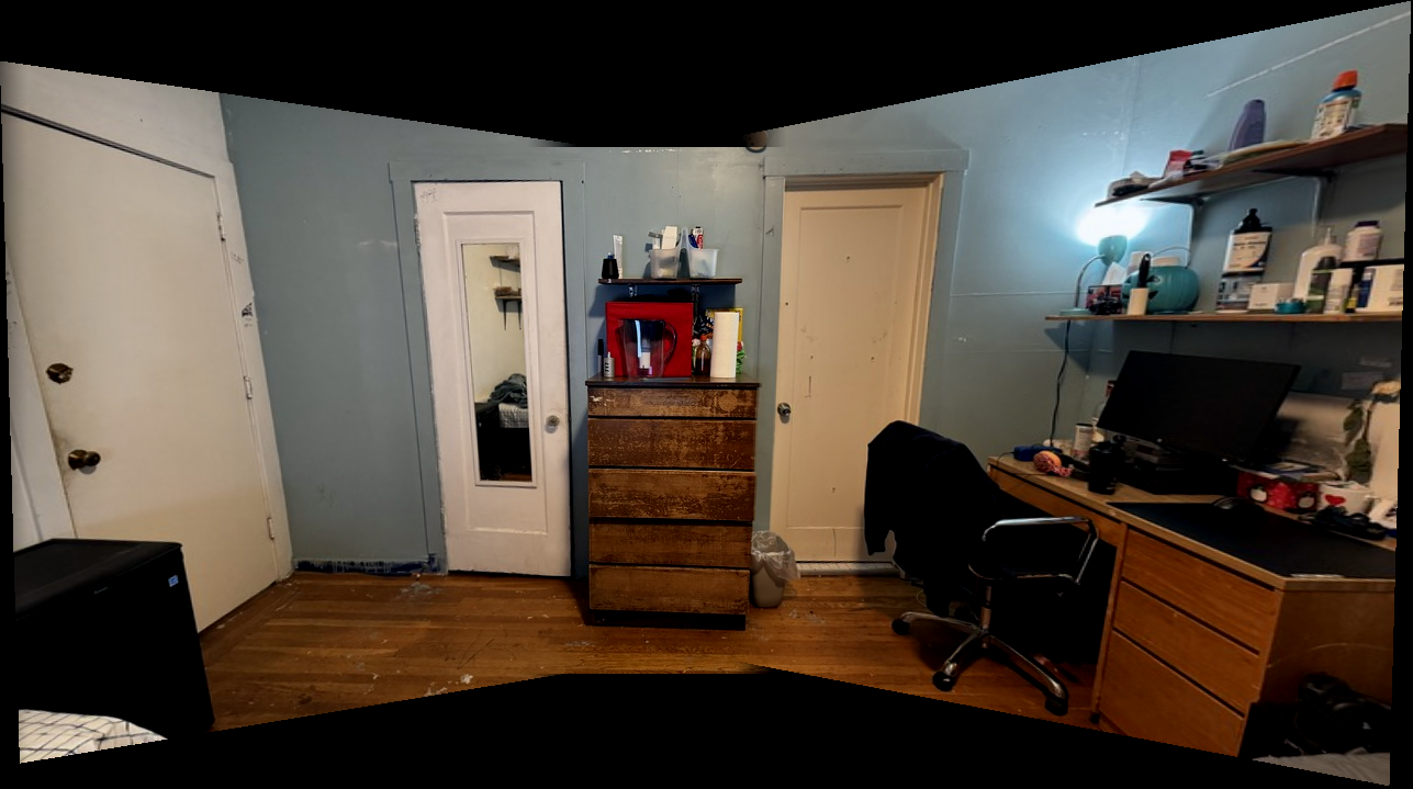
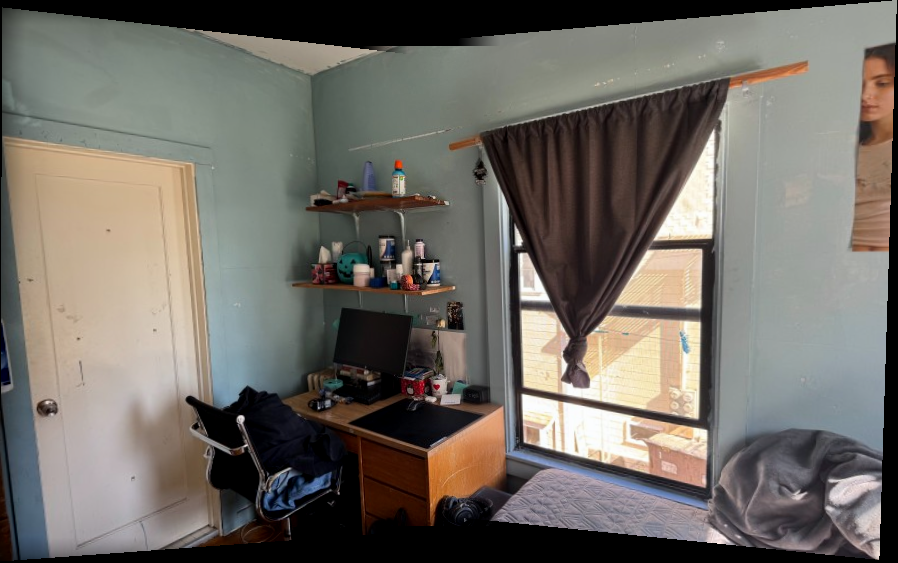
In this part of the project, the idea is to automatically detect corners in the image, form correspondences between pairs of images, and then select the best correspondences for the most stable homographies. This way, we don't have to manually select the correspondence points.
In the first step, we want to find some points that generally resemble corners as these will provide a strong starting point for discovering correspondences. To do this, we use the Harris corner detector (provided to us in the spec), which returns a number of candidate corner points, as well as the 'corner-y-ness' of each pixel in the image. I decided to use a black and white image to detect the corners as that was suggested in the spec. I ended up with around 6600 corners.
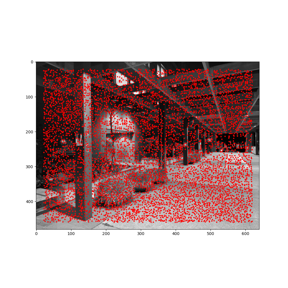
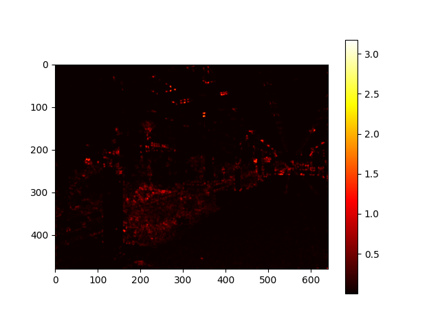
We can see that the heatmap makes sense since it seems to follow the basic geometry of the image - the shape of the image kind of slants towards the right side.
For this step, we extract the strongest corners that are not too close to other "strongest" corners, in essentials. We start by sorting the candidate points in descending order of their strength values, obtained from the Harris strength array. It then calculates pairwise distances between all points using the dist2 helper function. For each point in this sorted list, the function calculates a "suppression radius" (r-value), which is the minimum distance to any previously processed point with a strength value that exceeds a fraction (c_robust) of the current point's strength. This ensures that only points that are sufficiently strong and spatially distinct from stronger points are retained. After calculating the suppression radius for each point, the points are ranked by their r-values. The larger the r-value, the stronger of a corner that point is (because its strength is greater than all the other candidates within that radius). Optionally, we can take the top-k points from this ordered list instead of just returning the entire thing. I chose to take only the top 200 ANMS points, shown below.
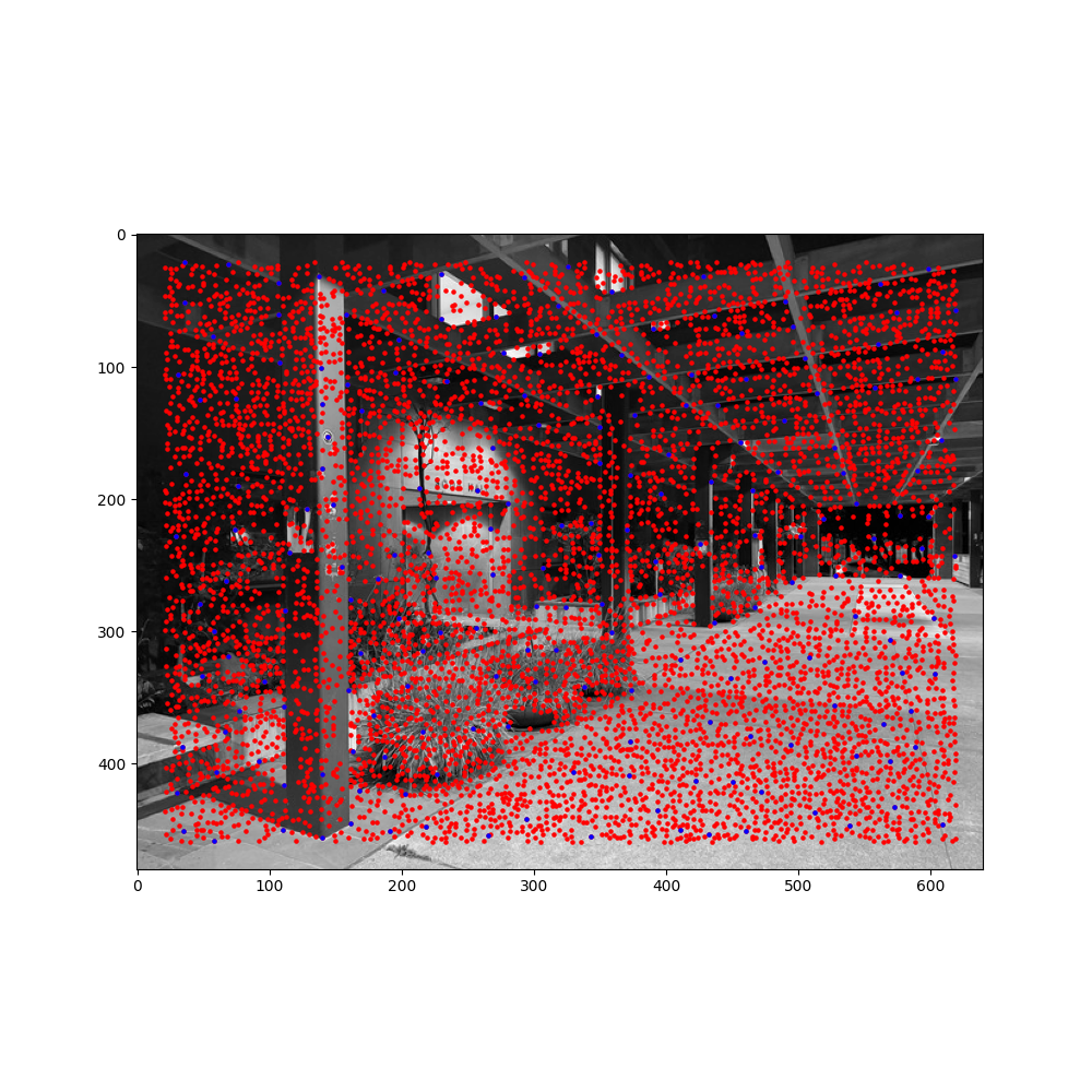
The overall idea is that we want to find corresponding corners between images. To do this, we need to find a way to match the corners from one image to another. We need to match corners that look similar to each other because those will probably become correspondences. We can collect features for each corner by sampling a 40x40 patch centered at each corner, and down-sampling (Gaussian blurring) that to an 8x8 patch which extracts the relevant features of that corner. We then normalize this 8x8 feature map by subtracting the mean and dividing by the standard deviation.
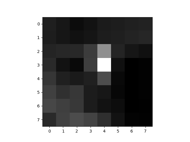
After doing steps 1-3 for two images, we now have k (number of ANMS corners) feature descriptors for each image. We now need to match corners that have similar feature maps, since these probably correspond to the same corners in the images. First, we calculate the pairwise distances between image 1's descriptors and image 2's descriptors. Then, for each descriptor in image 1, we take the 2 best descriptors from image 2. We then use Lowe's thresholding technique - If the first nearest neighbor is at least 2 times better (threshold of 0.5) than the second nearest neighbor, then that means it's likely to be an actual match, so we add that to our list of matches. In practice, from the 200 corners outputted by ANMS, I whittled it down to 31 likely correspondences using this technique.
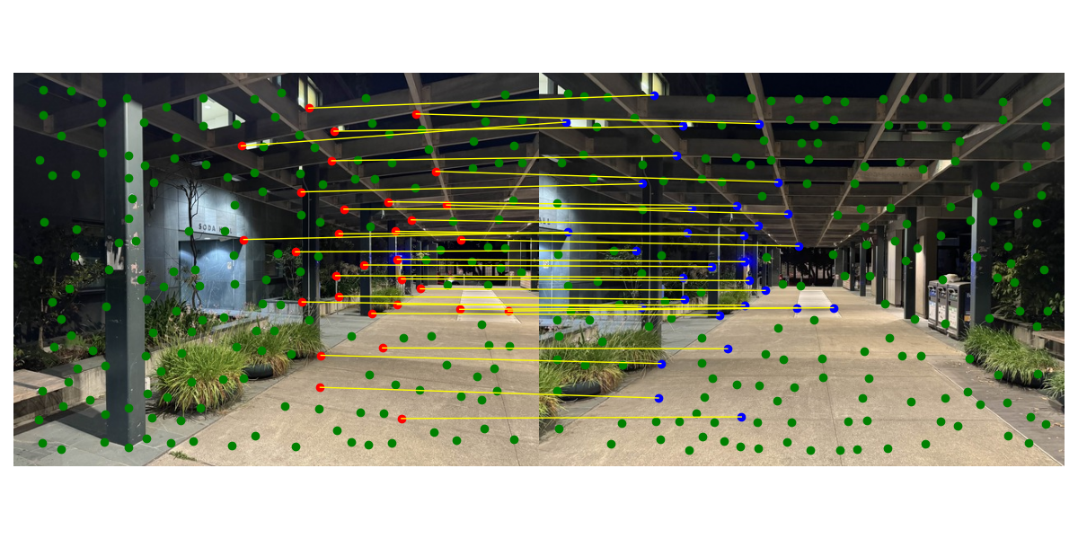
We are approaching the end of this process. We want the best possible correspondences to compute the most robust homography. If we just use all of the points from the process above, some of the correspondences will be wrong, and since the homography calculation (least squares) is not robust to outliers, it will damage the homography calculation. In the 4-point RANSAC algorithm, we select 4 random correspondences and compute a homography for that random sample. Then, we apply that homography to the other correspondences to see if it transforms them correctly. If the Euclidean distance between actual point in image 2 and the transformed point (from applying the homography to image 1's point) is less than some threshold, then this correspondence is an "inlier" meaning that the current homography worked for that correspondence. Essentially, we keep sampling over thousands of iterations until we stop, and then our new homography will be the one that had the most inliers. The inliers are the correspondences that we will use now, all the other correspondences will be discarded. In practice I used 4000 RANSAC iterations with a threshold of 1 to achieve the best results.
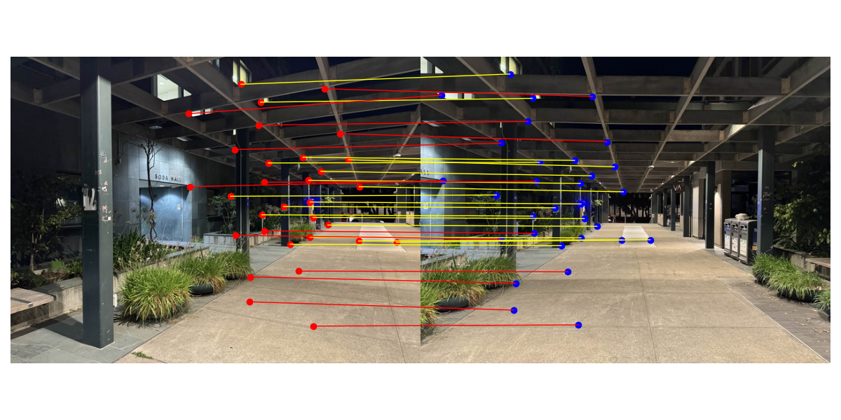
Now that we have our homographies, we can use the code from part 4a to warp the images and create the mosaics. Here are the 3 examples I chose.

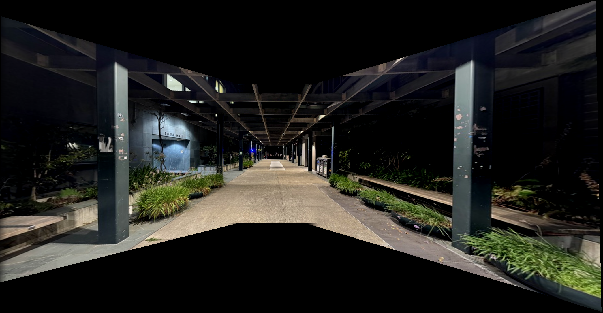

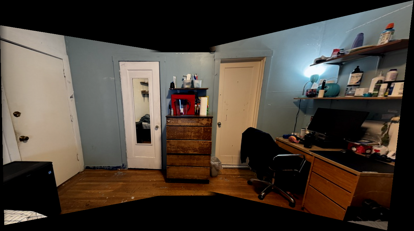

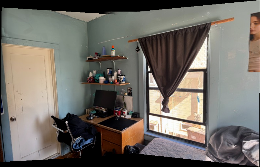
Arguably, some of the automatically generated panoramas look better than the manually generated ones! If we compare the Soda Hall mosaics, the manual one has some of the pillars slanted while the automatic one keeps them upright instead. Something new I learned about while doing this project is the Adaptive Non-Maximal Suppression algorithm. This might be the most interesting thing in this project, and implementing the function was a fun puzzle to figure out. RANSAC was also an interesting concept - it seems so intuitive, straightforward, and brute-forcey, but it did pull out the best correspondences. Sometimes the simplest algorithm is best!